Pull the Data

library(tidyverse)

employed <- read_csv("https://raw.githubusercontent.com/rfordatascience/tidytuesday/master/data/2021/2021-02-23/employed.csv")
employed %>% glimpse()

## Rows: 8,184
## Columns: 7
## $ industry         <chr> "Agriculture and related", "Agriculture and related"…
## $ major_occupation <chr> "Management, professional, and related occupations",…
## $ minor_occupation <chr> "Management, business, and financial operations occu…
## $ race_gender      <chr> "TOTAL", "TOTAL", "TOTAL", "TOTAL", "TOTAL", "TOTAL"…
## $ industry_total   <dbl> 2349000, 2349000, 2349000, 2349000, 2349000, 2349000…
## $ employ_n         <dbl> 961000, 58000, 13000, 94000, 12000, 96000, 931000, 1…
## $ year             <dbl> 2020, 2020, 2020, 2020, 2020, 2020, 2020, 2020, 2020…

Clean the Data

Define a helper function

show_column_elements <- function(data, var) {
  var <- enexpr(var)
  data %>% pull(!!var) %>% unique() %>% sort()
}

and run

employed %>% show_column_elements(industry)

employed %>% show_column_elements(major_occupation)

employed %>% show_column_elements(minor_occupation)

employed %>% show_column_elements(race_gender)

skimr::skim(employed)

You will see why we need to clean the data as follows.

employed <- employed %>% 
  filter(
    !industry %in% c(show_column_elements(employed, race_gender), NA)
  ) %>% 
  mutate(
    industry = case_when(
      industry == "Mining, quarrying, and\r\noil and gas extraction" ~
        "Mining, quarrying, and oil and gas extraction",
      TRUE ~ industry
    ),
    minor_occupation = case_when(
      minor_occupation == "Manage-ment, business, and financial operations occupations" ~
        "Management, business, and financial operations occupations",
      TRUE ~ minor_occupation
    )
  )

Aggregate the Data

Use industry and minor_occupation to define occupation, group the data by occupation and race_gender, and compute the average number of employees in 2015-2020 for each group.

library(glue)

employed_aggregated <- employed %>% 
  group_by(
    occupation = glue("{industry} | {minor_occupation}"),
    race_gender
  ) %>%
  summarise(n = mean(employ_n)) %>%
  ungroup()

employed_aggregated

## # A tibble: 1,254 x 3
##    occupation                                        race_gender               n
##    <glue>                                            <chr>                 <dbl>
##  1 Agriculture and related | Construction and extra… Asian                3.33e2
##  2 Agriculture and related | Construction and extra… Black or African Am… 1.00e3
##  3 Agriculture and related | Construction and extra… Men                  1.18e4
##  4 Agriculture and related | Construction and extra… TOTAL                1.22e4
##  5 Agriculture and related | Construction and extra… White                1.05e4
##  6 Agriculture and related | Construction and extra… Women                3.33e2
##  7 Agriculture and related | Farming, fishing, and … Asian                1.33e4
##  8 Agriculture and related | Farming, fishing, and … Black or African Am… 3.27e4
##  9 Agriculture and related | Farming, fishing, and … Men                  7.55e5
## 10 Agriculture and related | Farming, fishing, and … TOTAL                9.56e5
## # … with 1,244 more rows

Preprocess the Data for Clustering

Say we are interested in demographic groups “Black or African American”, “Asian”, and “Women”, and filter the data by these groups. Then, we put the data into a wide format, filter out some minority occupations, and compute the demographic distribution for each remaining occupation.

employment_wide <- employed_aggregated %>% 
  filter(
    race_gender %in% c("Black or African American", "Asian", "Women", "TOTAL"),
  ) %>%
  pivot_wider(names_from = race_gender, values_from = n, values_fill = 0) %>% 
  janitor::clean_names() %>% 
  select(occupation, black_or_african_american, asian, women, total) %>% 
  filter(total > 1e4) %>% 
  mutate(
    across(c(-occupation, -total), ~ .x / total)
  )

employment_wide

## # A tibble: 185 x 5
##    occupation                          black_or_african_a…   asian  women  total
##    <glue>                                            <dbl>   <dbl>  <dbl>  <dbl>
##  1 Agriculture and related | Construc…             0.0822  0.0274  0.0274 1.22e4
##  2 Agriculture and related | Farming,…             0.0342  0.0139  0.211  9.56e5
##  3 Agriculture and related | Installa…             0.0309  0.0155  0.0103 3.23e4
##  4 Agriculture and related | Manageme…             0.00867 0.00996 0.259  1.04e6
##  5 Agriculture and related | Office a…             0.0155  0.0233  0.841  8.58e4
##  6 Agriculture and related | Producti…             0.104   0.0332  0.185  3.52e4
##  7 Agriculture and related | Professi…             0.0373  0.0339  0.329  4.92e4
##  8 Agriculture and related | Protecti…             0.0682  0       0.136  1.47e4
##  9 Agriculture and related | Sales an…             0.0213  0       0.426  1.57e4
## 10 Agriculture and related | Service …             0.0334  0.00557 0.388  8.98e4
## # … with 175 more rows

Now, we can already gain some insights by sorting the data by your demographic group of interest. For example

library(DT)

employment_wide %>%
  arrange(-asian) %>%
  datatable(
    options = list(
      pageLength = 5,
      columnDefs = list(list(className = 'dt-center', targets = 2:5))
    )
  ) %>%
  formatRound(columns = c("black_or_african_american", "asian", "women"), digits = 2) %>%
  formatRound(columns = c("total"), digits = 0)

Next, we scale the data (for numerical reasons) to get it ready for k-means clustering.

employed_transformed <- employment_wide %>% 
  mutate(
    across(where(is.numeric), ~ scale(.x) %>% as.numeric())
  )

K-Means Clustering

We use the following plot to determine that 5 clusters will be used for the k-means algorithm

library(broom)

tibble(k = 1:20) %>% 
  mutate(
    kclust = map(
      k, 
      ~ kmeans(
        select(employed_transformed, -occupation), 
        centers = .x, nstart = 10
      )
    ),
    glanced = map(kclust, glance)
  ) %>% 
  unnest(glanced) %>% 
  ggplot(aes(k, tot.withinss)) +
  geom_line(alpha = 0.8) + 
  geom_point(size = 2) + 
  geom_vline(xintercept = 5, col = "red", alpha = 0.5)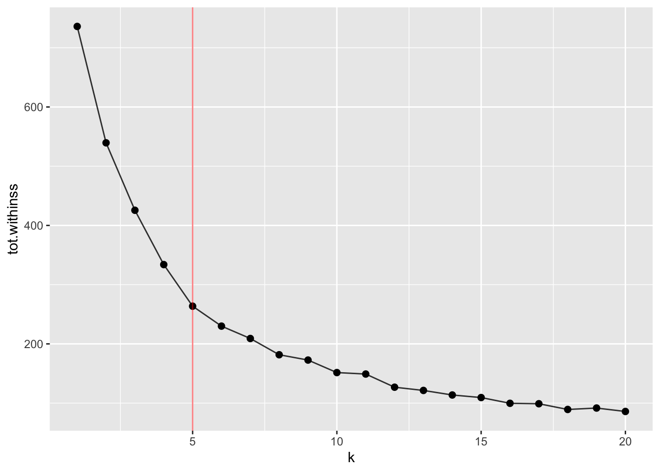

because k = 5 seems to be the elbow point. To fully understand how this plot is made, you need to know:

1. Functional programming and the {purrr} package

2. The glance() function from the {broom} package (tidy() and augment() are also good to know)

3. list-column

4. nest() and unnest() from the {tidyr} package

Then, we can go ahead and run the k-means clustering algorithm and visualize the result as follows. Notice that, besides Black or African American and Asian attributes, Women is mapped to the size of a point.

p <- kmeans(
  select(employed_transformed, -occupation), centers = 5, nstart = 10
) %>% 
  augment(employed_transformed) %>% 
  ggplot(
    aes(
      x = asian, y = black_or_african_american, size = women,
      col = .cluster, name = occupation)
  ) +
  geom_point(alpha = 0.4) + 
  labs(x = "Asian", y = "Black or African American")

plotly::ggplotly(p)

Also notice that the ggplotly() function from the {plotly} package can be used to convert a ggplot object to a plotly object, which allows you to hover your mouse over individual data points to see more details.

Now, you can draw your own conclusion on how race and gender impact occupation clustering by reading and touching this interactive plot.